This artical was original from https://medium.com/@sahiluppal/bag-of-freebies-95092859d279
The author owns the copyright of the article.
A list of techniques used in combination to improve a variety of computer vision task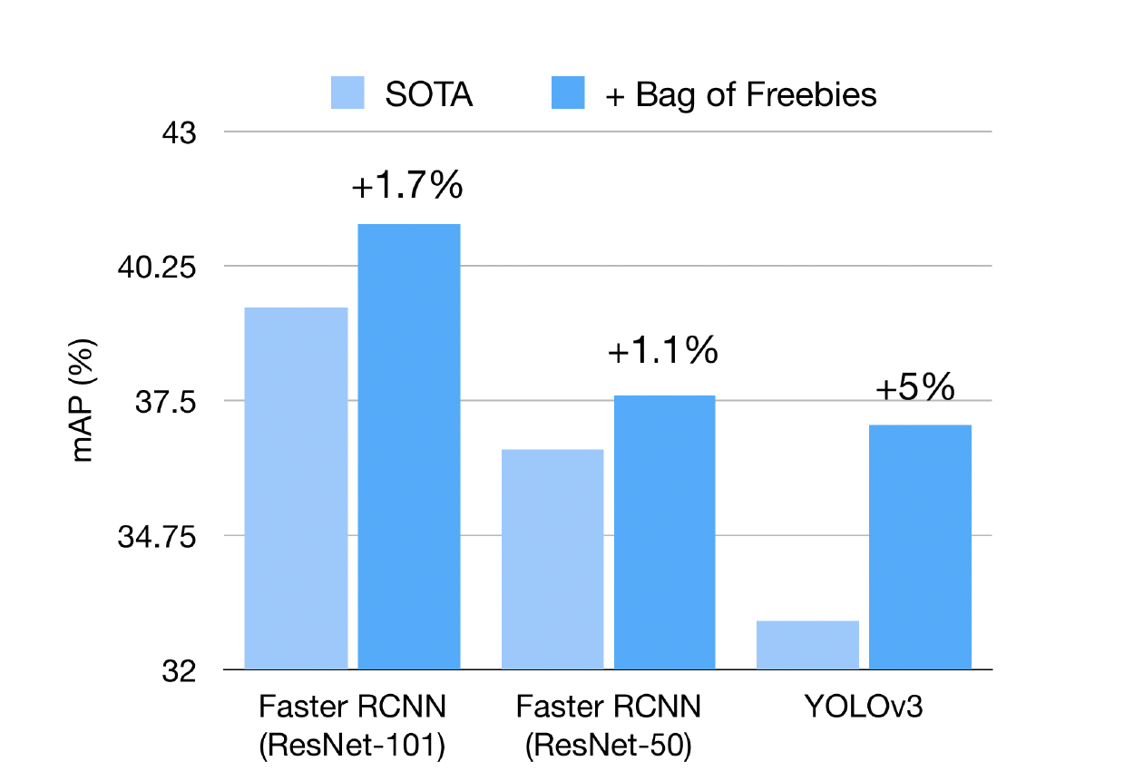
Object detection is, no doubt, one of the most fundamental applications in computer vision. Latest state-of-the-art detectors (including single-stage like YOLO or multiple-stage like RCNN [and derivatives]) are based on image classification backbone networks e.g., VGG, ResNet etc.
There are multiple techniques “collectively known as Bag of Freebies”, which can be used in combination to boost the performance of all popular object detection networks without introducing extra computational cost during inference.
Why Bag of Freebies got attention?
Usually, object detectors are trained offline. Therefore, researchers always like to take advantage and develop better training methods which can make the object detector receive better accuracy without increasing inference cost. These methods only changes the training strategy or what we can say training cost. You can think bag of freebies as a pipeline of data augmentation techniques. The sole purpose of data augmentation is to increase the variability of the input images, so that the designed object detection model has higher robustness to the images obtained from different environments.
In general, photometric distortions and geometric distortions are two commonly used data augmentation method and they definitely benefit the object detection tasks. In photometric distortions, we adjust the brightness, contrast, hue, saturation and noise of an image. For geometric distortions, we add random scaling, cropping, flipping, and rotating. In addition, some researchers engaged in data augmentation put their emphasis on simulating object occlusion issues (when an object covers a portion of another object.).
These freebies are all training time modifications, and therefore, only affect model weights without changing the network structure and have achieved good results in image classification and object detection methods.
Bag of Freebies
In this section, we enlist an image mix-up method for object detection. We will introduce data processing and training schedule designed to improve performance of object detection models.
1. Image Mix-up for Object Detection
The key idea of mix-up in image classification task is to linearly mixing up pixels from one image to another image in a specific ratio where both images belong to the same training dataset. At the same time, one-hot encoded labels of both images are also mixed using the same ratio. The ratio in mix-up algorithm is drawn from a distribution called beta distribution written as B(alpha, beta).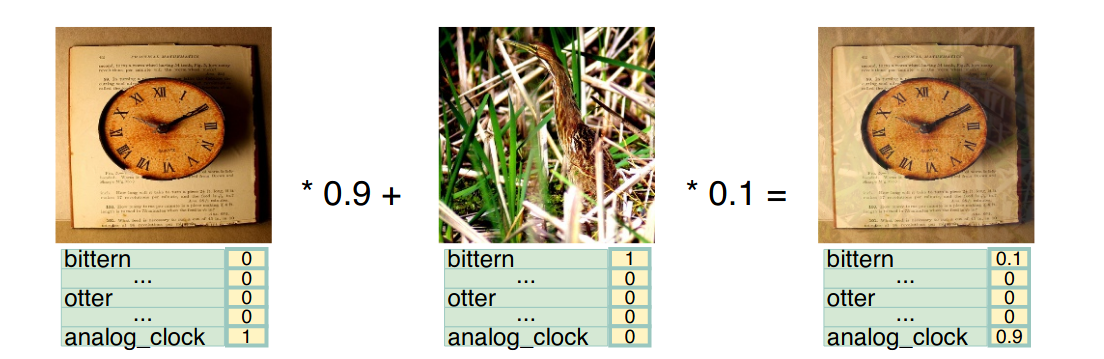
//small
Mix-up visualization of image classification with typical mix-up ratio of 0.1: 0.9. Two images are mixed uniformly across all pixels, and image labels are weighted summation of original one-hot label vector.
In this example, a bird image is mixed with a wall clock image in a typical 0.1: 0.9 ratio and so as their one-hot encoded labels.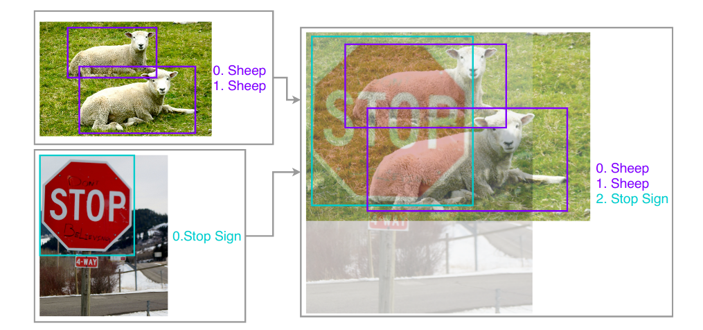
//small
Geometry preserved alignment of mixed images for object detection. Image pixels are mixed up, object labels are merged as a new array.
In this example, both images are merged along with their ground truth object coordinates as a new array while preserving their geometry.
To verify mix-up designed for object detection, while choosing a beta distribution with alpha, beta are both at least 1,we experimentally test mix-up ratio distributions using the YOLOv3 network on Pascal VOC dataset. Below Table shows the actual improvements by adopting detection mix-up ratios sampled by different beta distributions. Beta distribution with alpha and beta both equal to 1.5 is marginally better than 1.0 equivalent to uniform distribution). It increases the mean average precision by almost 3% from the baseline.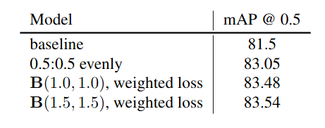
//small
Effect of various mix-up approaches, validated with YOLO3 on Pascal VOC 2007 test set. Weighted loss indicates the overall loss is the summation of multiple objects with ratio 0 to 1 according to image blending ratio they belong to in the original training images.
In contrast, Rosenfeld conducted a series of experiments name as “Elephant in the room”, where an elephant image patch is randomly placed on a natural image, then this adversarial image is used to challenge existing object detection models. The results indicate that existing object detection models are prune to such attack and show weakness to detect such transplanted objects. Researchers followed the same experiments by sliding an elephant image patch through an indoor room image, trained two YOLOv3 models on COCO 2017 dataset with one mix-up approach and other isn’t. They can observe that vanilla model trained without mix-up approach is struggling to detect “elephant in the room” due to heavy occlusion and lack of context because it’s rare to capture an elephant in a kitchen, and model trained with mix approach is more robust. In addition, they also noticed that mix model is more humble. less confident and generates lower scores for object on average. However, this behavior does not affect evaluation results as shown.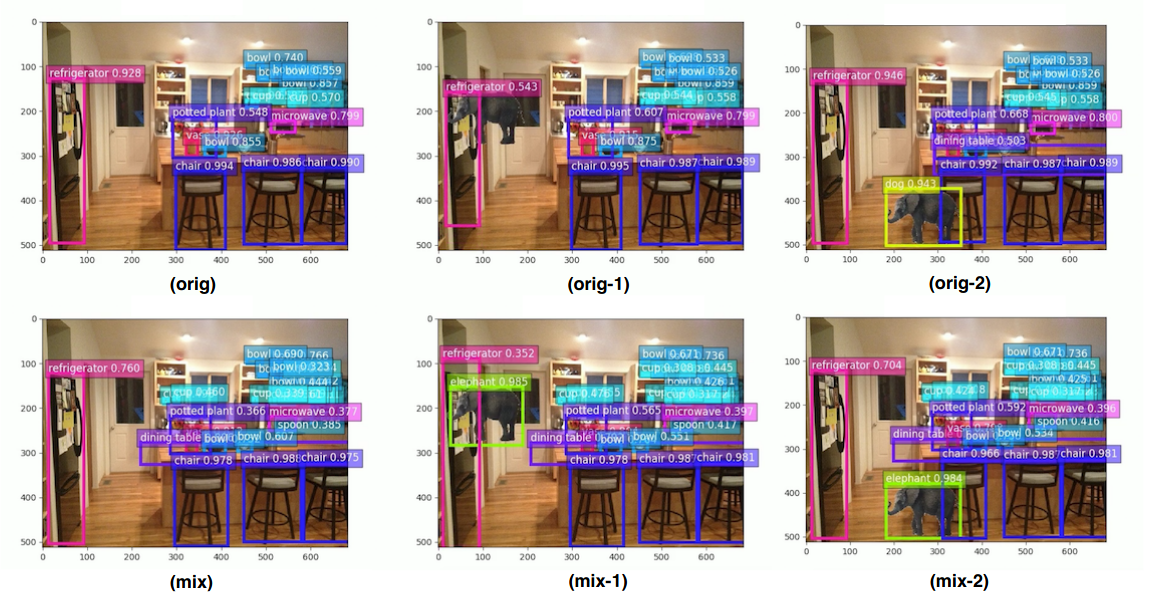
//small
Elephant in the room example. Model trained with geometry preserved mixup (bottom) is more robust against alien objects compared to baseline (top)
It was obvious that model trained with visually coherent mixup is more robust (94.12 vs 42.95) to detect elephant in indoor scene even though it is very rare in natural images. And even mix-up model easily handles occlusion as you can see in bottom row. The mix-up model receives more challenges during training therefore is significantly better than vanilla model in handling unprecedented scenes and very crowded object groups.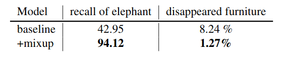
/small
Statistics of detection results affected by elephant in the room. ”Recall of elephant” is the recall of sliding elephant in all generated frames, indicating how robust the model handles objects in unseen context.
2. Classification Head Label Smoothing
Label smoothing is a loss function modification that has been shown to be very effective for training deep learning networks. Label smoothing improves accuracy in image classification, translation, and even speech recognition. The simple explanation of how it works is that it changes the training target for the neural nets from a hard ‘1’ to ‘1-label smoothing adjustment’, meaning the neural nets is trained to be a bit less confident of it’s answers.
Example: assume we want to classify images into dogs and cats. If we see a photo of a dog, we train the neural nets (via cross entropy loss) to move towards a 1 for dog, and 0 for cat. And if a cat, the reverse where we train towards 1 for cat, 0 for dog. In other words, a binary or “hard’ answer.
However, neural nets have a bad habit of becoming ‘over-confident’ in their predictions during training, and this can reduce their ability to generalize and thus perform as well on new, unseen future data. In addition, large datasets can often include incorrectly labeled data, meaning inherently the neural nets should be a bit skeptical of the ‘correct answer’ to reduce extreme modeling around some degree of bad answers.
Thus, what label smoothing does is force the neural nets to be less confident in it’s answers by training it to move towards the ‘1-adjustment’ target, and then dividing the adjustment amount over the remaining classes…. rather than simply a hard 1.
For our binary dog/cat example, label smoothing of .1 means the target answer would be .90 (90% confident) it’s a dog for a dog image, and .10 (10% confident) it’s a cat, rather than the previous move towards 1 or 0. By being a bit less certain, it acts as a form of regularization and improves it’s ability to perform better on new data.
Label smoothing’s affect on Neural Networks: Now we get to the heart of the paper, which shows visually how label smoothing affects the NN’s classification processing.
ResNet classifying “airplane, automobile and bird” during training and validation.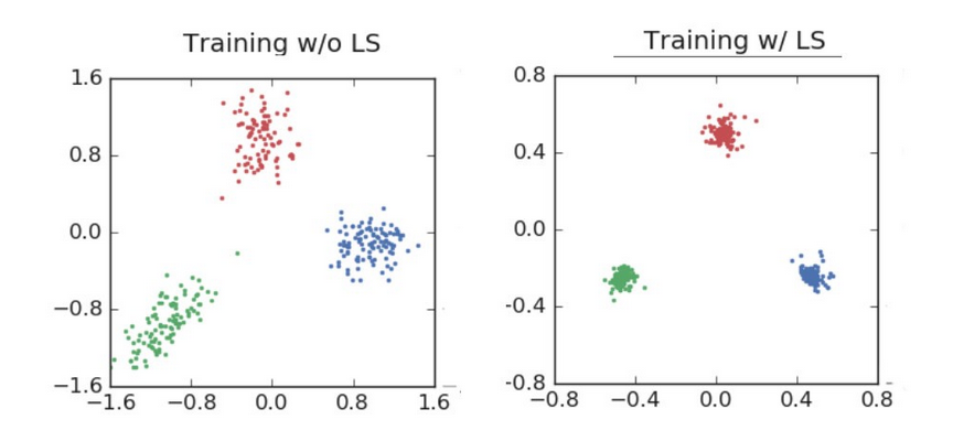
// small
ResNet training for classifying 3 image categories…note the tremendous difference in cluster tightness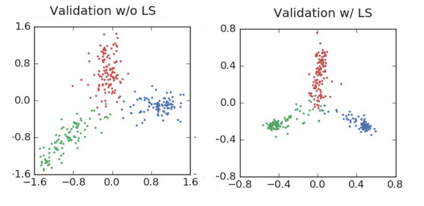
// small
ResNet validation results. Label smoothing increased the final accuracy. Note that while the label smoothing drives activations to tight clusters in training, in validation it spreads around the center and leverages a full range of confidences with it’s predictions.
As the images visually show, label smoothing produces tighter clustering and greater separation between categories for the final activations.
This is a primary reason why label smoothing produces more regularized and robust neural networks, that importantly tend to generalize better on future data. However, there’s an additional beneficial effect than just better activation centering.
3. Data Preprocessing
In image classification domain, usually neural networks are extremely tolerant to image geometrical transformation. It is actually encouraged to randomly augment the images e.g. randomly flip, rotate and crop images in order to improve generalization accuracy and avoid overfitting.
In terms of types of detection networks, there are two type of pipelines for generalizing final predictions. First is single stage detector networks, where final outputs are generated directly from feature map from the CNN backbone, for example SSD(single shot detector) and YOLO networks. The second type is multi-stage proposal and sampling based approaches, following Fast-RCNN, where a certain number of regions are sampled from a large pool of generated ROIs, where final outputs are generated by applying cropping based techniques to the feature maps from CNN backbone.
Since multi-stage networks already applies cropping based techniques, they doesn’t need their input to be augmented with random cropping and many more extensive geometric augmentations. But single stage detectors can reproduce highly appealing results if augmentation is applied to the input images. This is the major difference between one-stage and so called multi-stage object detection data pipelines.
4. Training Schedule Revamping
During training, the learning rate usually starts with a relatively big number and gradually becomes smaller throughout the training process. For instance the default learning rate schedule for Faster-RCNN is to reduce learning rate by ratio 0.1 to 60k iterations. Similarly, YOLOv3 uses same ratio 0.1 to reduce learning rate at 40k and 45k iterations. As this is a sharp learning rate transition which may cause the optimizer to re-stabilize the learning momentum in the next few iterations.
In contrast a smoother cosine learning rate adjustment can be used. Cosine schedules scales the learning rate according to the value of cosine function on 0 to pi.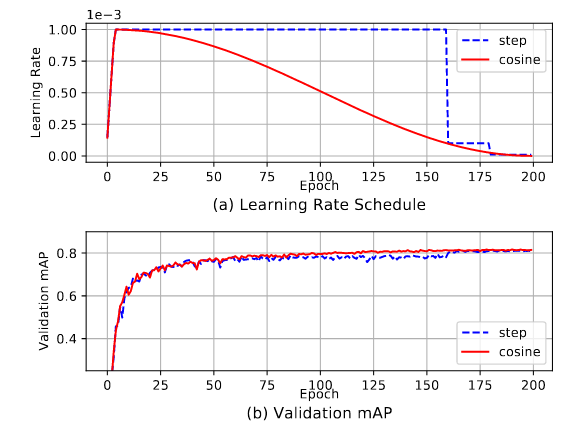
Visualization of learning rate scheduling with warmup enabled for YOLOv3 training on Pascal VOC. (a): cosine and step schedules for batch size 64. (b): Validation mAP comparison curves using step and cosine learning schedule.
Warmup learning rate is another common strategy to avoid gradient explosion during the initial training iterations. Training with cosine schedule and proper warmup lead to better validation accuracy as shown in the figure.
5. Synchronized Batch Normalization and Random Shape Input
Neural networks are compute intensive but are highly parallelizable. This leads us to the need of computation environments to equip multiple devices (GPUs) to accelerate training. Batch Normalization helps us to train input data in chunks while reducing sensitivity towards hyperparameters. Although the typical implementation of Batch Normalization working on multiple devices (GPUs) is fast, but experiments suggests that reducing size of batch size on multiple devices causing slightly different statistics during computation, which potentially degraded performance. This is not a significant issue in some standard vision tasks such as ImageNet classification (as the batch size per device is usually large enough to obtain good statistics). However, it hurts the performance in some tasks with a small batch size (e.g., 1 per GPU).
Natural training images come in various shapes. To fit memory limitation and allow simpler batching, many single-stage object detection networks are trained with fixed shapes. To reduce risk of overfitting and to improve generalization of network prediction, researchers follow YOLOv3’s official implementation details and used a mini-batch of N training images and resized to N x 3 x H x W, where H and W are multipliers of network stride. For example YOLOv3 use H = W = {320,352,384,416,448,480,512,544,576,608} for training using VGG as CNN backbone whose stride is 32.
Results
Stacking all these tweaks for object detection, researchers sticked to major frameworks YOLOv3(representing single-stage pipelines) which is famous for its efficiency and good accuracy and Faster-RCNN(representing multi-stage pipelines) which is one of the most adopted detection framework and foundation of many others variant.
YOLOv3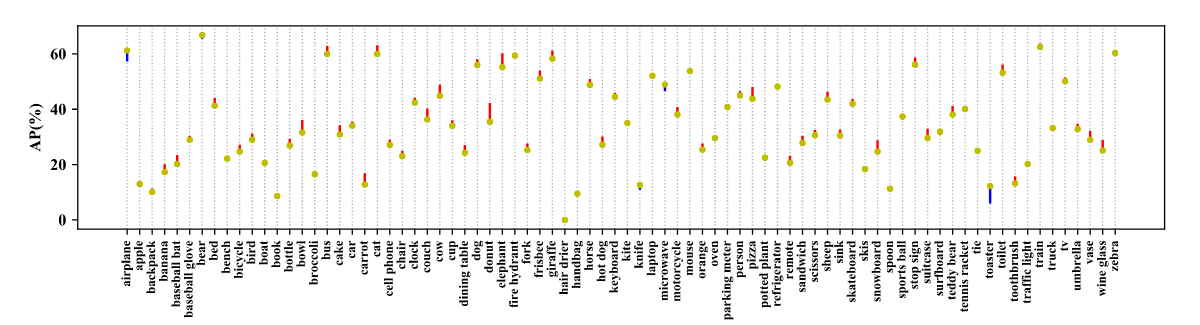
//small
->COCO 80 category AP analysis with YOLOv3 .Red lines indicate performance gain using bag of freebies, while blue lines indicate performance drop.<-
As we can see in the above representation, YOLOv3 is trained on COCO dataset on which have almost 80 categories. while using the above tweaks researchers can claim the performance gain (shown in red) and we can also see some performance drop (shown in blue). But overall YOLOv3 gets 3.43% performance gain on AP.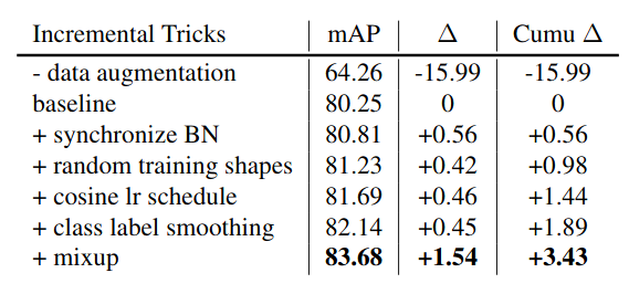
//small
Incremental trick validation results of YOLOv3, evaluatedat416×416on Pascal VOC 2007 test set.
Faster-RCNN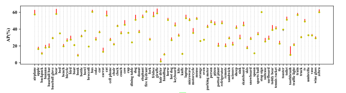
// small
COCO 80 category AP analysis with Faster-RCNN resnet50. Red lines indicate performance gain using bag of freebies, while blue lines indicate performance drop.
Similarly in the above representation, Faster-RCNN with ResNet50 CNN backbone also trained on COCO dataset. while using the above tweaks researchers can claim the performance gain (shown in red) and we can also see some performance drop (shown in blue). But overall Faster-RCNN gets 3.55% performance gain on AP.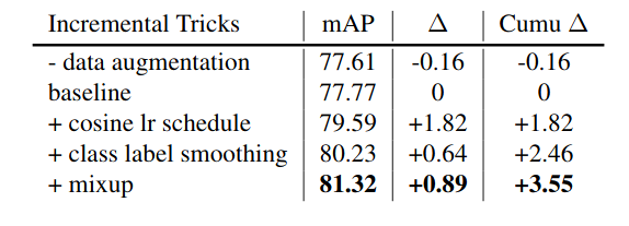
Conclusion
In this article, we showed that how bag of training enhancements significantly improves model performances while introducing zero overhead to the inference environment. Empirical experiments of YOLOv3 and Faster-RCNN on Pascal VOC and COCO datasets show that the bag of tricks are consistently improving object detection models. By stacking all these tweaks, we observe no signs of degradation of any level and suggest a wider adoption to future object detection pipelines. These freebies are all training time modifications and therefore only affect model weights without increasing inference time or change of network structures.
References
[1] Bag of Freebies for Training Object Detection Neural Networks. https://arxiv.org/pdf/1902.04103.pdf
[2] YOLOv4: Optimal Speed and Accuracy of Object Detection. https://arxiv.org/pdf/2004.10934.pdf
[3] Gluoncv toolkit. https://github.com/dmlc/gluon-cv
[4] Redmon and A. Farhadi. Yolov3: An incremental improvement. https://arxiv.org/abs/1804.02767
[5] Label Smoothing & Deep Learning: Google Brain explains why it works and when to use (SOTA tips). https://medium.com/@lessw/label-smoothing-deep-learning-google-brain-explains-why-it-works-and-when-to-use-sota-tips-977733ef020
[6] Faster R-CNN: Towards Real-Time Object Detection with Region Proposal Networks. https://arxiv.org/abs/1506.01497