In order to understand how parallel computing works, we have to understand a few concepts.
A multithreaded computation can be represetned by a Directed Acyclic Graph of vertices. Each vertex represents the executtion of an instruction.
First of all, let`s take a look at 2 concepts:
Cost model: Work and Span:
Work
The total work that will be executed by all the processors.
If we consider the whole process that a computer finish all the tasks as a Directed Acyclic Graph, then work is the total number of all vertices of the DAG.
Span: sometime we call it depth, is the length of the longest path of the
DAG(critical path).
See the picture below, work == 21, span == 8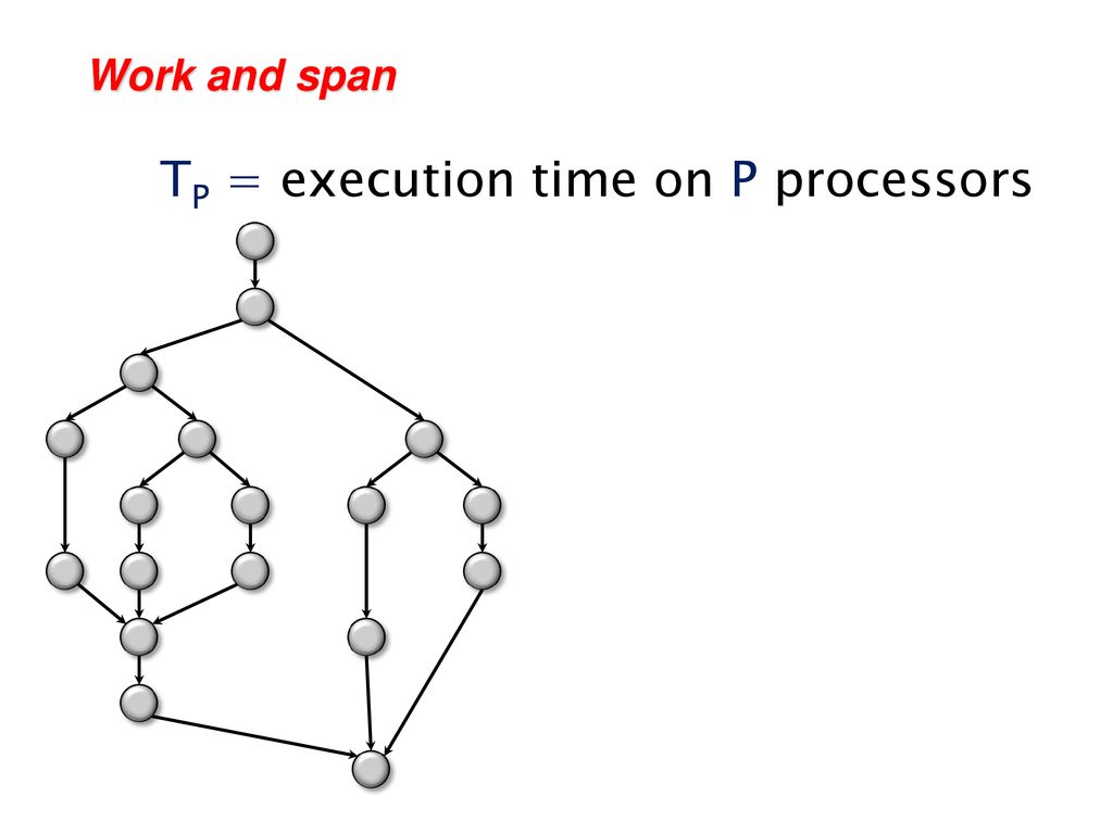
Brent`s Theorem:
Brent`s theorem is the theorem to give the upper bound and lower bound of the time that expires between the start of the computation and its end. Let us
denote it as Tp, denote total work as W, Span as D, number of processors as N.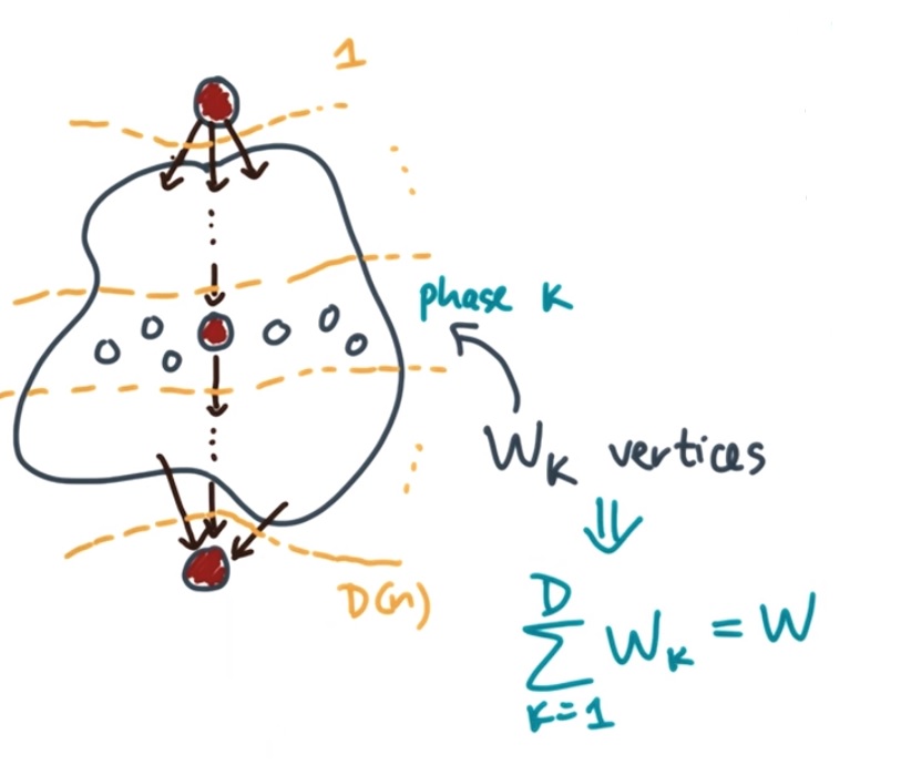
Then we can easily have:
Tp = ∑(1 to D)(floor(Wi-1)/P) + 1
based on the properties of ceiling and floor operation, we have
max(D, ceiling(W/N)) <= Tp <= (W-D)/N + D
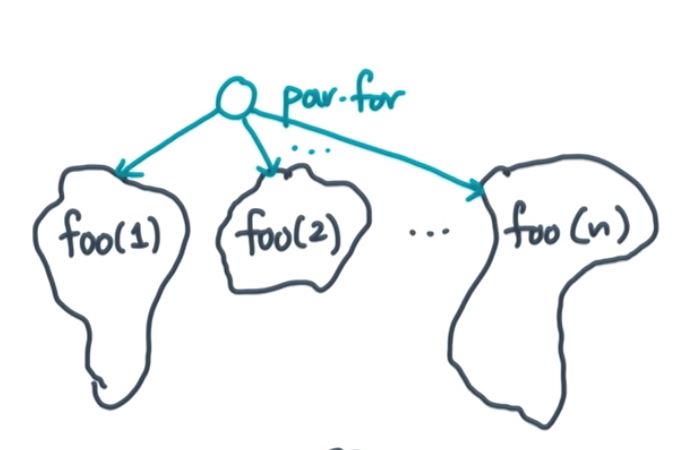
par-for loop:
(parallel for loop, sometimes people call it for-any loop or for-all loop)
All iterations are independent to each other.
The DAG above shows how does a offline scheduling problem works. In reality, we might don`t have full knowledge of the DAG. Instead, the DAG unfolds as we run the program. Futhermore, we are interested in not only minimizing the length of the schedule but also the work and time it takes to compute the schedule. These 2 conditions defin the online scheduling problem.